Rico Inf Curve
Particle streams in a four-singularity well, and the propellantless ship sized to the numbers.
Two bodies of in-house research share this page. The first is Rico Inf Curve: a Newtonian, GPU-accelerated study of high-density particle streams moving in the field of four fixed singularities, with hard-sphere ricochet at the horizon radius and long-time orbit classification. It covers verification of the physics, a batched integrator, a 99,856-particle production run, the geometry of the curves, a scan over spatial dimension, a time-reversibility experiment, an asymptotic-expansion check, and a separate geodesic module that answers the general-relativity questions properly. The second is EM-D Stream: three propellantless drive mechanisms, what was validated and at what significance, the negative results, and a crewed vehicle of 28.9 t sized to the measured plasma-magnet numbers.
The model
In normalised units, G = 1 and test mass m = 1, the softened four-centre potential per unit mass and the equations of motion are
\Phi(\mathbf r) = -G\sum_{i=1}^{4}\frac{q_i}{\sqrt{|\mathbf r-\mathbf r_i|^2+\varepsilon^2}},\qquad \dot{\mathbf r}=\mathbf v,\qquad \dot{\mathbf v} = -G\sum_i q_i\,\frac{\mathbf r-\mathbf r_i}{\left(|\mathbf r-\mathbf r_i|^2+\varepsilon^2\right)^{3/2}}The softening \varepsilon removes the 1/r divergence so the ODE stays integrable, and the constructor enforces \varepsilon \le R_{\min}/2 so the regularisation never reaches into the sampled region. The physical surface |\mathbf r-\mathbf r_i| = R_i is handled discretely. A terminal root-finding event stops the integration, the velocity is reflected specularly, and the integration restarts just outside:
\hat{\mathbf n} = \frac{\mathbf r-\mathbf r_i}{|\mathbf r-\mathbf r_i|},\qquad \mathbf v' = \mathbf v-(1+e)(\mathbf v\cdot\hat{\mathbf n})\,\hat{\mathbf n}\quad\text{for } \mathbf v\cdot\hat{\mathbf n}<0With e = 1 the ricochet is elastic and conserves energy exactly, which makes energy drift a clean diagnostic of integrator quality rather than a mix of physics and numerics. The production geometry is the tetrahedron: four centres of charge +1 at (±0.577, ±0.577, ±0.577) with an even number of minus signs, horizon radius 0.05 and softening 0.001. Two further geometries ship as controls, a planar square with alternating ±q and a true 1/r³ far field, and a collinear arrangement with an exact mirror symmetry.
H = |\mathbf p|^2/2m + m\Phi(\mathbf r) in flat space. There is no metric tensor, no light cone, no proper time and no event horizon in any relativistic sense. The horizon here is a hard sphere, a numerical regularisation chosen to keep the ODE integrable near the centres. The general-relativity results further down come from the geodesic module, a separate program that shares no physics code with the stream integrator.Verification
The inherited scaffold had never been executed. The verification suite runs nine groups of checks, 20 assertions in all: the analytic gradient against central differences, the tidal tensor against a numerical Hessian, the quadrupole far-field exponent, the Kepler limit, energy conservation, the elastic ricochet, and mirror symmetry. All 20 passed on the first execution with no tolerance loosened.
| Check | Result |
|---|---|
| Analytic gradient against central differences | max rel. err 1.62×10⁻¹⁰ |
| Tidal tensor against numerical Hessian | max rel. err 4.31×10⁻¹⁰, asymmetry exactly 0 |
| Planar quadrupole far field | fitted exponent 3.000 |
| Kepler closure after 10 periods | 4.71×10⁻⁷ relative |
| Kepler energy drift | 2.31×10⁻¹¹ |
| Four-centre energy drift (t = 120) | 2.68×10⁻⁹ |
| Elastic ricochet speed | 6.167651 in, 6.167651 out (< 10⁻⁹) |
| Mirror symmetry (collinear) | 0.00, bit-exact |
The GPU integrator
A serial CPU solver integrates one particle per call, and a stream of 10⁵ particles is 10⁵ serial solves. The field is static and identical for every particle, so the ensemble is embarrassingly parallel. The replacement is a batched Dormand-Prince 5(4) in PyTorch in which every particle carries its own adaptive step and its own event state. The ensemble advances in lockstep at the level of kernel launches, not simulated time: one particle can take 10⁻⁶ steps near a horizon while another coasts at 10⁻¹ in the far field, in the same kernel.
The discontinuous ricochet is what makes this non-trivial. The four horizon surfaces and the escape sphere are folded into one continuous scalar,
G(y) = \min\Big(\min_i\big(|\mathbf r-\mathbf c_i|-R_i\big),\; R_{\rm esc}-|\mathbf r|\Big)positive in the physical region and negative once anything is crossed, so a single root-finder serves all five surfaces and which one fired is decided afterwards from which term attained the minimum. The root is bracketed across the accepted step and refined with Illinois regula falsi in which every trial evaluation is a real RK5 step, not an interpolant, so the located crossing carries the integrator's own order of accuracy. Steps are clamped so a particle lands exactly on the output grid, and the whole thing runs in float64: the shadow-orbit separation for the Lyapunov measurement starts at 10⁻⁸ against coordinates of order 1, which float32 cannot resolve.
Validation against the CPU reference found three bugs: a conflated step-clamping flag that let a particle's clock run ahead of its physics, a Zeno trap in the proximity cap that made a horizon unreachable, and retired particles being re-flushed every iteration. Chaotic trajectories cannot be compared at long times, so the comparison is layered by what is legitimately comparable: field kernels to 3.2×10⁻¹⁶, Kepler over ten periods to 1.64×10⁻⁸, a five-bounce ricochet to 3.50×10⁻⁶, a chaotic orbit at t = 20 to 1.89×10⁻¹⁰, and the long-time CPU-to-GPU divergence measured to grow as exp(0.210 t), the system's own Lyapunov rate.
| N | wall | ms/iter | particles/s | speedup |
|---|---|---|---|---|
| 1,024 | 32.9 s | 10.2 | 31 | 6.2× |
| 4,096 | 59.0 s | 17.7 | 69 | 13.7× |
| 16,384 | 119.7 s | 33.6 | 137 | 27.1× |
| 65,536 | 171.1 s | 48 | 383 | 75.8× |
| 262,144 | 206.4 s | 49.8 | 1,270 | 251× |
The production run
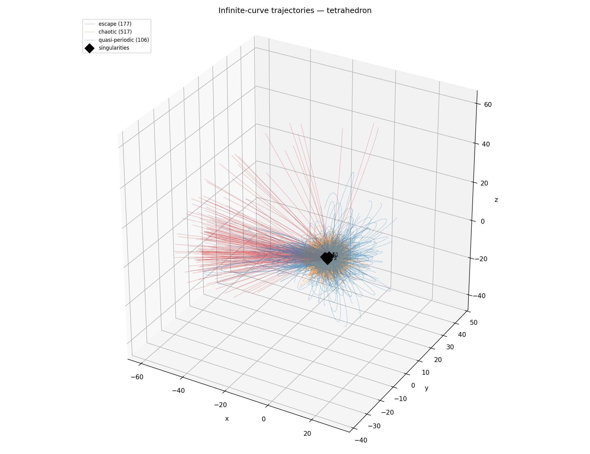
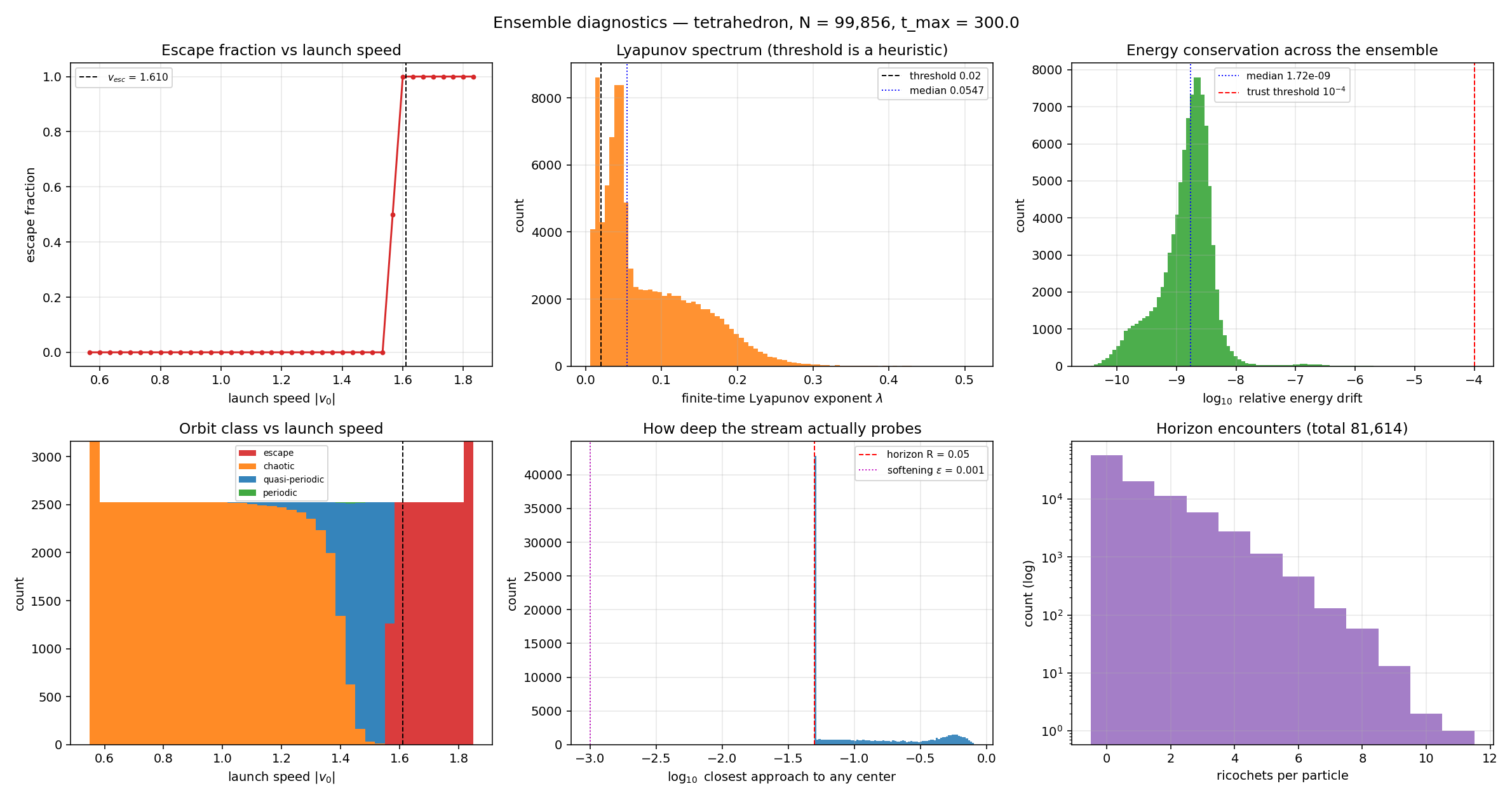
99,856 particles were integrated to t = 300 in 1,108 s: 15,600 GPU loop iterations totalling 655,885,314 RK steps, of which 1.66% were rejected by the error controller. The stream launches from (3.0, 0.4, 0.6) into a cone of half-angle 0.30 rad about (−1, −0.13, −0.2) with speeds swept across 0.55 to 1.85. The local escape speed at the launch point is 1.6097, so the ensemble deliberately straddles it.
| Class | Count | Share |
|---|---|---|
| chaotic | 64,631 | 64.7% |
| escape | 22,120 | 22.2% |
| quasi-periodic | 13,070 | 13.1% |
| periodic | 35 | 0.035% |
Curve geometry and the dimensional scan
A dedicated run integrated 384 curves in the tetrahedron potential to t = 600 at rtol = 10⁻¹¹ with 24,000 samples each, so that the geometry of the paths themselves could be measured. All 384 stayed bounded. They made 806 ricochets between them, and the median turning angle at a cusp was 86.2°. The box-counting dimension of the curve set came out at D = 2.17, which is what a family of space-filling rosettes with occasional sharp cusps should give: more than a line, well short of a surface.
Taking the question of dimension seriously cannot mean keeping a 1/r potential and adding coordinates. A point source in D spatial dimensions obeys Laplace's equation, whose Green's function gives
\Phi(r)\sim -\frac{1}{r^{D-2}}\ \ (D\ge 3),\qquad \Phi(r)\sim +\ln r\ \ (D=2),\qquad V_{\rm eff} = \frac{L^2}{2r^2}+\Phi(r)so the force falls as 1/r^(D−1). For a central force r^(−n) circular orbits are linearly stable only when n < 3, so stable bound orbits require D < 4. At D = 4 both terms of the effective potential scale as 1/r² and there is no minimum at all; for D ≥ 5 the attraction wins at small r and the extremum is a maximum. Setting D = 3 reproduces the original module to 1.78×10⁻¹⁵, checked on every run. These are extra spatial dimensions in a flat metric, not a second time dimension and not compactified circles.
| D | force ∝ | stable annulus | four-centre bound |
|---|---|---|---|
| 2 | r⁻¹ | 100% | 75.3% |
| 3 | r⁻² | 100% | 44.3% |
| 4 | r⁻³ | 2.7% | 2.3% |
| 5 | r⁻⁴ | 0% | 0.1% |
| 6 | r⁻⁵ | 0% | not reported |
| 7 | r⁻⁶ | 0% | not reported |
Reversibility
The equations are invariant under t → −t with v → −v: acceleration depends only on position, so reversing every velocity retraces the path exactly, and elastic specular reflection is its own inverse. The microscopic laws here have no arrow of time. The experiment integrates forward to T, negates every velocity, integrates forward another T, and measures how close each particle comes to its starting point. 256 particles, elastic horizons, rtol = 10⁻¹².
| T | median | p90 | max |
|---|---|---|---|
| 5 | 1.52e-12 | 2.95e-12 | 7.53e-12 |
| 20 | 2.47e-11 | 1.34e-10 | 3.24e-9 |
| 40 | 2.90e-10 | 5.77e-9 | 7.38e-7 |
| 60 | 2.27e-9 | 2.77e-7 | 1.03e-4 |
| 80 | 1.92e-8 | 1.17e-5 | 7.81e-3 |
| 100 | 1.85e-7 | 3.60e-4 | 7.45e-1 |
| 140 | 1.25e-5 | 1.06e+0 | 6.28e+0 |
| 180 | 3.83e-4 | 4.21e+0 | 6.71e+0 |
\text{recovery error}\ \approx\ 2.05\times10^{-12}\;\exp\!\big(0.0550\cdot 2T\big)At T = 5 the round trip returns every particle to within 1.5×10⁻¹². By T = 180 the median particle misses its own starting point by 3.8×10⁻⁴ and the worst misses by 6.7 length units, a distance comparable to the whole configuration. The fitted amplification rate is 0.0550 per unit time. The independently measured median Lyapunov exponent of the 99,856-particle ensemble is 0.0547. Those two numbers come from different measurements, one from shadow-orbit divergence in the forward problem and one from a forward-and-back round trip, and they agree to better than 1%. The practical reversibility horizon is T ≈ 182: beyond it the past is arithmetically unrecoverable at double precision even though it remains mathematically determined, and recovering a further factor of e in time costs a factor of e^0.11 in precision.
The asymptotic check
The far-field test in the verification suite fits one number, the slope of log|Φ| against log r, and asserts that it is 3.000. That checks the leading exponent and no coefficient at all. The structure being claimed is an asymptotic series in 1/r from the Legendre generating function,
\Phi(\mathbf r) = -G\sum_{\ell}\frac{M_\ell(\hat{\mathbf n})}{r^{\ell+1}},\qquad M_\ell(\hat{\mathbf n}) = \sum_i q_i\, r_i^{\ell}\, P_\ell(\hat{\mathbf n}\cdot\hat{\mathbf r}_i)and the testable consequence is that truncating after the leading term must leave a residual falling as 1/r^(ℓ+2), with the coefficient matching the analytic moment. The tetrahedron has no dipole moment and no quadrupole moment: its four vertex vectors satisfy \sum_i \hat{\mathbf r}_i\otimes\hat{\mathbf r}_i = \tfrac{4}{3}I, which is isotropic, so \sum_i P_2(\hat{\mathbf n}\cdot\hat{\mathbf r}_i) = 0 identically. The leading correction to its monopole is the octupole at 1/r⁴, measured as a residual decaying at r⁻⁴ after monopole subtraction, with M₃ = 2.1659. The planar closed form M₂ = 3a²(nₓ² − n_y²) is reproduced to 4.4×10⁻¹⁶, and all odd moments vanish to 1.1×10⁻¹⁶ by inversion symmetry.
| Configuration | M₀ | M₁ | M₂ | First correction | Measured residual |
|---|---|---|---|---|---|
| planar alternating | 0 | 0 | 3a²(nₓ² − n_y²) | M₄ (hexadecapole) | r⁻⁵ |
| tetrahedron | 4q | 0 | 0 | M₃ (octupole), M₃ = 2.1659 | r⁻⁴ |
| collinear | 4q | 0 | 4.3182 | M₂ (quadrupole) | r⁻³ |
The relativistic questions and the geodesic module
The questions that motivated this work were relativistic: how time becomes space inside a horizon, why an infalling body never seems to cross, what happens to curvature at the centre. None of them can be answered by the Newtonian integrator, so a separate program was written. It shares no physics code with the stream integrator; only the numerics carry over, the same Dormand-Prince stepping, per-particle adaptive steps and event root-finding. The state is (x^\mu, u^\mu) in R⁸ and the law is the geodesic equation,
\frac{du^\mu}{d\tau} = -\Gamma^\mu_{\alpha\beta}\,u^\alpha u^\beta,\qquad g_{\mu\nu}u^\mu u^\nu = -1,\qquad E=-u_t,\quad L=u_\phiMetrics implemented: Schwarzschild, Painlevé-Gullstrand and ingoing Eddington-Finkelstein, both horizon-regular, and Kerr in Boyer-Lindquist coordinates with frame dragging and an ergosphere. Christoffel symbols come two ways, closed-form for Schwarzschild and a fully general numeric path from central differences of the metric, and the two agree to 2.97×10⁻¹¹. That agreement is what makes the module extensible: any metric written as a function of position gets correct geodesics without hand-derived formulas. Units are G = c = 1 with M = 1, so the horizon sits at r = 2.
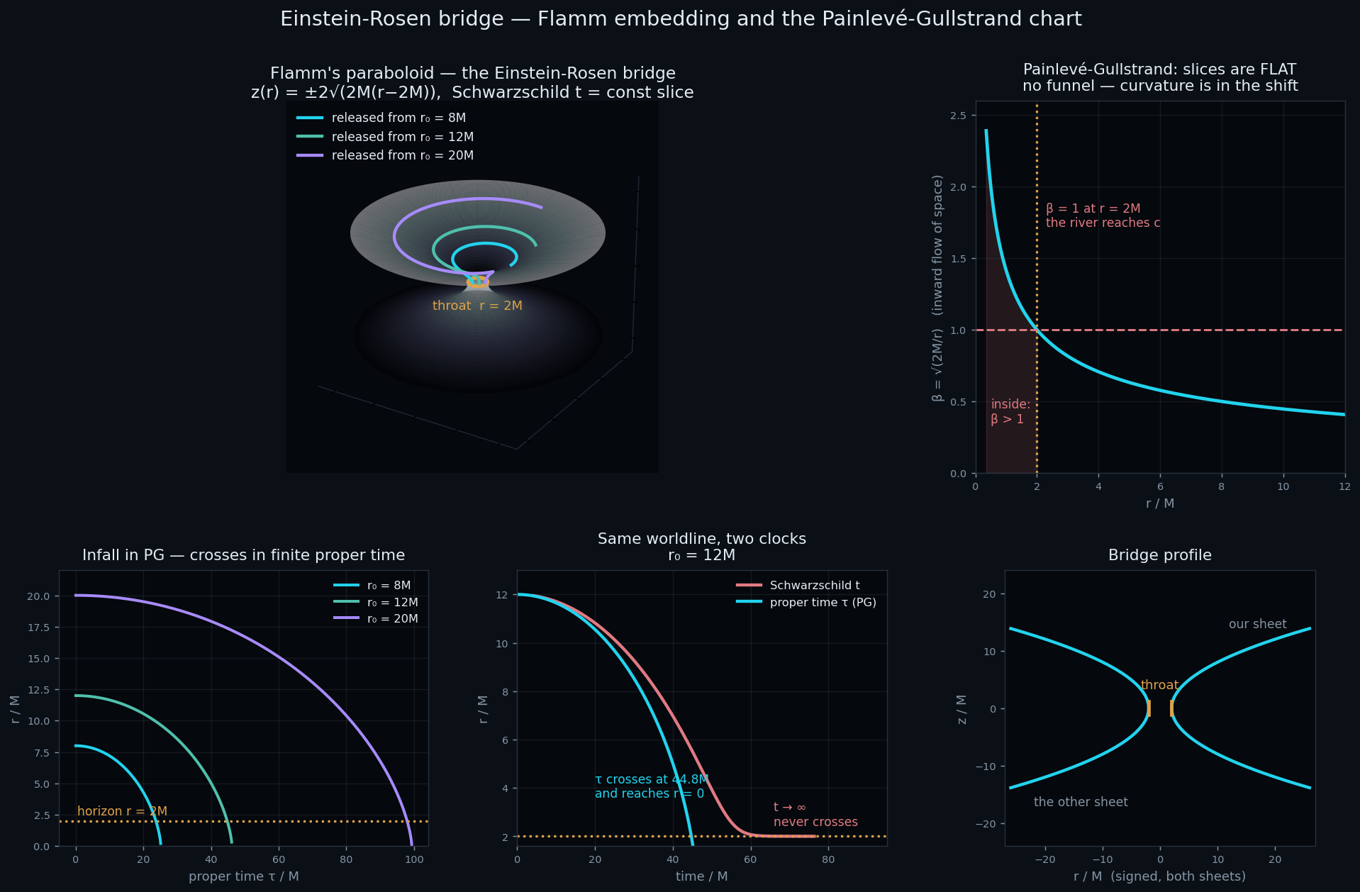
The same infall in two charts
A body released from rest at r₀ = 10M, integrated in two charts of the same spacetime. In the Schwarzschild chart, the distant static observer's clock, r_min = 2.000000118. It never crosses. Coordinate time diverges logarithmically: stopping successively closer gives t = 47.17, 51.91, 56.53, 61.16 and 65.76 for r − 2M = 10⁻¹ down to 10⁻⁵, a fitted slope of 2.0166 in −ln(r/2M − 1) against the predicted 2M = 2. In the Painlevé-Gullstrand chart, the infalling observer's clock, the same body crosses without incident and reaches r = 9.98×10⁻⁴ in proper time 35.124058650 against the exact
\tau = \pi\sqrt{\frac{r_0^3}{8M}} = 35.124058748,\qquad \text{relative error } 2.79\times10^{-9}Both are correct. The horizon is a property of the chart, not of the spacetime, and the disagreement is the answer rather than a paradox.
Time becoming space, measured
Inside r = 2M the metric components swap sign: g_tt = +1.000 and g_rr = −1.000 at r = M, so r is timelike and t is spacelike. The measured consequence: of 64 worldlines launched with a spread of angular momenta and initial radial kicks in both directions, 56 crossed the horizon, and every one of them had dr/dτ < 0 throughout the interior, with a maximum of −0.896. Not one moved outward, including those fired outward. The algebra behind it is that inside the horizon (uʳ)² ≥ |f| > 0, so uʳ can never reach zero and cannot change sign. The four-velocity norm holds to 8.66×10⁻¹¹ while crossing the horizon and stopping at r = 1, and degrades to 2.62×10⁻² stopping at r = 10⁻³: the integration error is concentrated entirely at r = 0, not at r = 2M, which is the statement that the horizon is regular and the singularity is not.
The turning-point cubic
With u = 1/r the radial equation becomes a cubic in u,
\text{timelike:}\ \left(\frac{du}{d\phi}\right)^{2} = \frac{E^2-1}{L^2} + \frac{2M}{L^2}u - u^2 + 2Mu^3,\qquad \text{null:}\ \left(\frac{du}{d\phi}\right)^{2} = \frac{1}{b^2} - u^2 + 2Mu^3Depressing the null cubic with u = w + 1/(6M) gives the roots in closed form,
u_k = \frac{1}{6M}\left(1 + 2\cos\frac{\theta - 2\pi k}{3}\right),\quad k = 0,1,2,\qquad u_0+u_1+u_2 = \frac{1}{2M}three roots 120° apart in the cosine argument. The roots in u sum to 1/(2M) to 12 digits, which proves that when all three are positive the third root always lies outside the horizon, since u₃ < 1/(2M) means r₃ > 2M. An initial assertion that it lay inside was wrong, and the algebra corrected it. Given E and L, the cubic recovers r_apo = 120 and r_peri = 80 to 10⁻⁹. The null double root is the photon sphere: b_crit = 3√3 M = 5.196152422706632 exactly, and integration measures the capture threshold at 5.19498, a relative error of 2.26×10⁻⁴. The ISCO is a triple root: at r = 6M all three roots coincide. Measured independently by perturbing circular orbits, r = 5.90 plunges to the horizon and r = 6.10 stays inside a band of 6.0915 to 6.1083. The Newtonian model has no capture cross-section because its horizon reflects; the geodesic module has one, 27πM², the b_crit disc, derived rather than imposed.
Verification of the module
Ten groups, all passing, each against a closed form that exists independently of the code: perihelion precession at 3.0×10⁻⁴ against the exact elliptic integral (the weak-field 6πM/p is 4.7% low at p = 96, so testing against it would have been testing the approximation), light deflection at 1.5×10⁻² and 7.8×10⁻³ of 4M/b, and the Newtonian limit recovering Kepler to 7.5×10⁻⁴ at r = 2000M.
EM-D Stream
A propellantless vehicle pairing a laboratory-validated plasma magnet with a reflector-shaped radiating array, operated sequentially rather than simultaneously.
Three propellantless drive mechanisms were investigated and simulated. Two are validated. They are complementary rather than competing, and a vehicle carrying two of them retains control authority in every operating environment. The document of record is the design specification, Rev D, dated 20 August 2026. Rev C presented the magnetic-sail mechanism as an open question requiring particle-in-cell validation. It is not open: Slough (IEPC-2007-015, 2007) reports a scaled laboratory experiment in which the mechanism was measured directly. Rev D restates the design on those measurements, withdraws one claim that did not survive quantitative check, and reduces the vehicle mass by an order of magnitude.
What it is
| A · Radiating array | B · Magnetic sail | C · Sequential induction | |
|---|---|---|---|
| Mechanism | reflector-shaped EM radiation | solar-wind momentum intercept | travelling-wave induction |
| Thrust | 2.76 mN per MWe | 3.8 N at 30 km, 12.7 N at 55 km | 11.4 N at n = 10¹⁸ |
| Requires | nothing | solar wind | ambient plasma |
| Propellant | none | none | scavenged |
| Vectoring | differential firing | coil orientation | firing sequence |
| Status | validated here | validated in lab (Slough) | validated here, 8.1σ |
| Quantity | Measured | Significance here |
|---|---|---|
| RMF-driven plasma current | > 10 kA | the bubble inflates |
| Thrust, ballistic pendulum | 2 N | direct force measurement |
| Equivalent jet power | about 1 MW | from a 50 km/s wind source |
| Plasma detachment | none observed | force reacted onto the antennas |
| Antenna radius / mass / power | 100 m / 20 kg / 100 W | replaces a 2.2 t coil |
| Achieved dipole scale | > 30 km | sets the thrust |
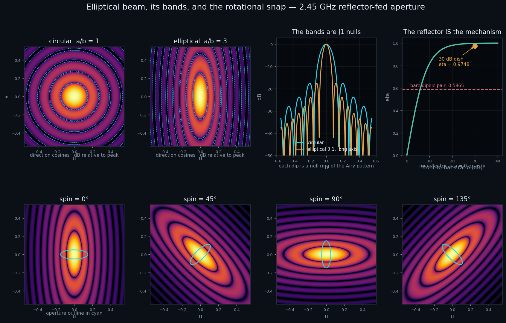
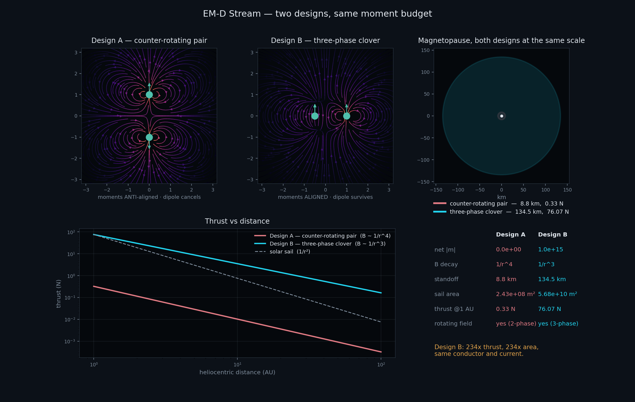
Contributed by this work: the reflector finding, that a bare aperture radiates a symmetric J₁ pattern and gives η = 0 exactly while a 30 dB reflector gives η = 0.9748, so the reflector is the entire mechanism rather than an improvement to it; sequence vectoring, that thrust direction follows firing order and not amplitude ratio, at 8.1σ with sign reversal across zero delay; the sequential architecture, in which sail and array never run simultaneously and so never fight; the hull structural limit of about 3×10⁷ A·m² per dynamo for a 2.2 m hull, from the Maxwell traction map; and a corrections register of fourteen documented errors and their mechanisms.
Validated results and negative results
| Claim | Measured | Significance |
|---|---|---|
| Sequential firing produces directed thrust | 5.42×10⁻²⁰ kg·m/s | 8.1σ |
| Thrust direction follows firing order | sign reversal | 7.0σ / 8.1σ |
| Symmetric control returns zero | 4.27×10⁻²¹ kg·m/s | 0.47σ, pass |
| Energy transferred by induction | +2638 eV per particle | direct |
| Aligned ring forms field-reversed core | z = ±R/√2 | 4 d.p. |
| Radiating array, 30 dB reflector | η = 0.9748 | 97.5% of P/c |
| Contra-rotating pair | η = 0.3812 | does not cancel |
| Pull-mode force, two routes | agree to 6 s.f. | validated |
| Hull traction, fore vs aft | equal and opposite | stretches, no net force |
| Configuration | Result | Cause |
|---|---|---|
| Alternating ring (+ − + −) as intake | 0.000 m² acceptance | null channels are 2-D planes, zero measure |
| Uniform stretch-and-release | nothing above noise | breathing drives azimuthal E only |
| Amplitude-ratio thrust vectoring | nothing above noise | direction follows order, not ratio |
| Polarity alone for radiation asymmetry | η = 0 exactly | real amplitudes give a fore-aft symmetric pattern |
| Self-generated gravity well | requires 1.9×10⁸ T | and cannot pull its own source regardless |
Physics
Field-reversed core
Four aligned dipoles of moment m ẑ on a ring of radius R. On the axis,
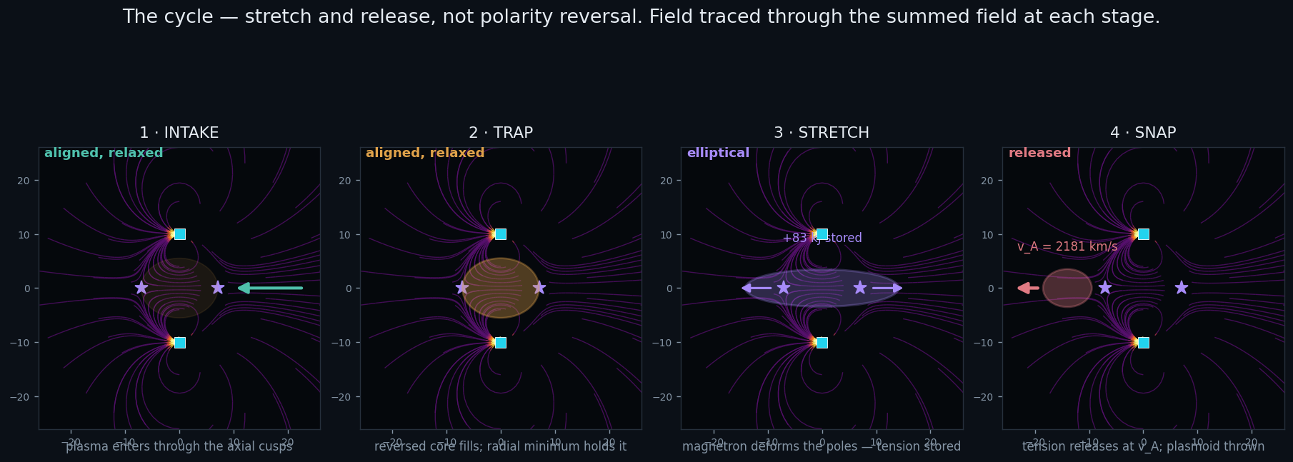
B_z(z) = n\,\frac{\mu_0 m}{4\pi}\,\frac{2z^2-R^2}{(R^2+z^2)^{5/2}}\quad\Longrightarrow\quad z_{\rm null} = \pm\frac{R}{\sqrt 2}independent of m and n. Predicted ±7.0711 m for R = 10 m and located numerically at ±7.0711 m. Between the nulls B_z < 0: the core field is reversed relative to the moments producing it. Measured |B| outward from the centre rises radially from 0.040 to 0.062 T, which confines, and falls to zero axially at the nulls, which is open. Confined radially and open axially is the structure of a nozzle, with the exhaust direction a property of the topology rather than something imposed. Because z_null depends only on geometry, current buys field strength and never field extent. In vacuum, hardware scale is topology scale, and a field structure larger than the hardware requires ambient plasma to carry the current.
Momentum transfer requires a translating pattern
Uniform amplitude modulation produces no thrust in any geometry tested. A dipole's vector potential is azimuthal, so ∂A/∂t is azimuthal, so the induced E is azimuthal: it spins plasma about the axis and cannot push it along the axis. Geometric asymmetry does not help, because the asymmetry resides in B while momentum transfer is performed by E. Axial momentum requires the field pattern to translate, which means rings fired in sequence.
Radiation momentum
\eta = \frac{\left|\oint I(\hat{\mathbf n})\,\hat{\mathbf n}\,d\Omega\right|}{\oint I(\hat{\mathbf n})\,d\Omega},\qquad F = \eta\,\frac{P_{\rm rad}}{c}\ \le\ \frac{P}{c} = 3.336\ \mu\mathrm{N/kW},\qquad \eta = \frac{1-r}{1+r}Since η ≤ 1, F ≤ P/c. This is not a modelling assumption: it is the momentum content of the electromagnetic field, U/c. A bare aperture radiates a J₁ pattern symmetric about its plane, so momentum cancels exactly and η = 0. Suppressing the back hemisphere by a front-to-back ratio r gives η = (1 − r)/(1 + r), and the reflector is the entire mechanism.
| Front-to-back ratio | η | N per kW radiated | % of photon limit |
|---|---|---|---|
| 0 dB (no reflector) | 0.00000 | n/a | 0.0% |
| 10 dB | 0.79916 | 2.666×10⁻⁶ | 79.9% |
| 20 dB | 0.95741 | 3.194×10⁻⁶ | 95.7% |
| 30 dB (design point) | 0.97480 | 3.252×10⁻⁶ | 97.5% |
Force requires an open circuit
\oint I\, d\mathbf l\times\mathbf B = I\left(\oint d\mathbf l\right)\times\mathbf B = 0Integrating dF = I dl × B around a closed loop in a uniform field gives exactly zero, verified numerically at 1 to 20 m radius and 1 to 100 kA at machine precision in every case. A closed loop obtains a torque, not a force. To obtain force the current must not return through the vehicle: an open conductor whose circuit closes externally. In space the only available conductor is ambient plasma.
Hull traction
Maxwell stress resolved over the hull surface by spherical angle. Cant angle controls the distribution: at 0° cant 15% of the hull is in tension; at 40°, 51%; at 90°, 58%. Peak tension rises from 8.9 to 57.7 kPa across that sweep. Forward and aft hemispheres are equal and opposite at every angle to five significant figures. The hull is stretched, not moved. Grid convergence on the residual confirms second-order convergence to zero, a ratio of 4.00 per doubling, identifying it as quadrature error.
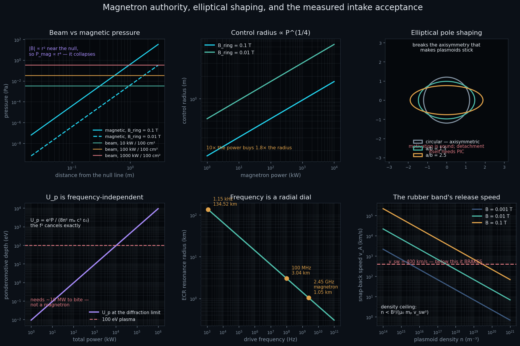
Mechanism figures
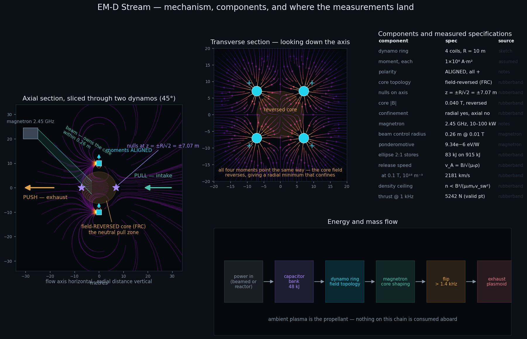
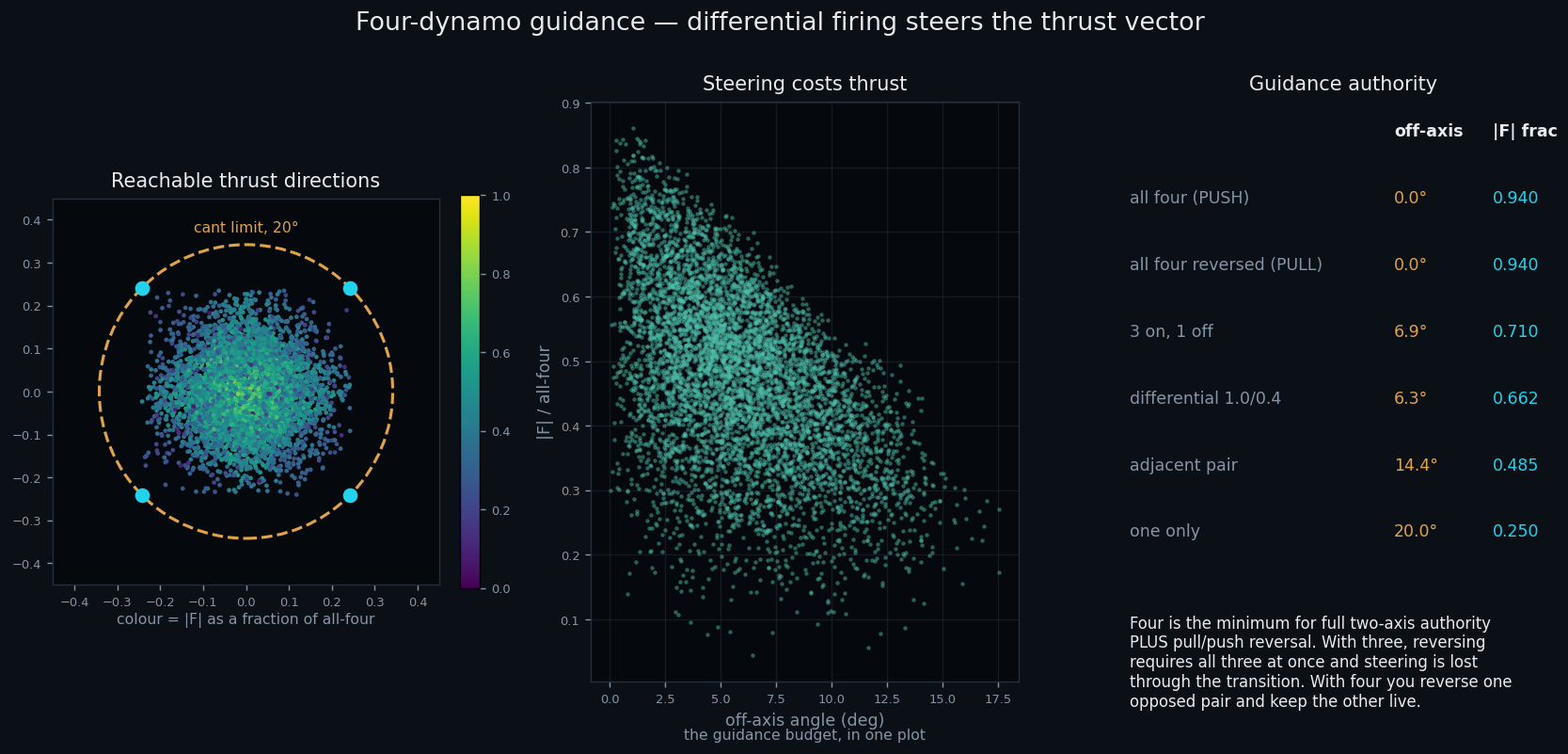
| Firing pattern | Off-axis | |F| fraction |
|---|---|---|
| All four (push) | 0.0° | 0.940 |
| All four reversed (pull) | 0.0° | 0.940 |
| Three on, one off | 6.9° | 0.710 |
| Adjacent pair | 14.4° | 0.485 |
| One only | 20.0° | 0.250 |
The vehicle
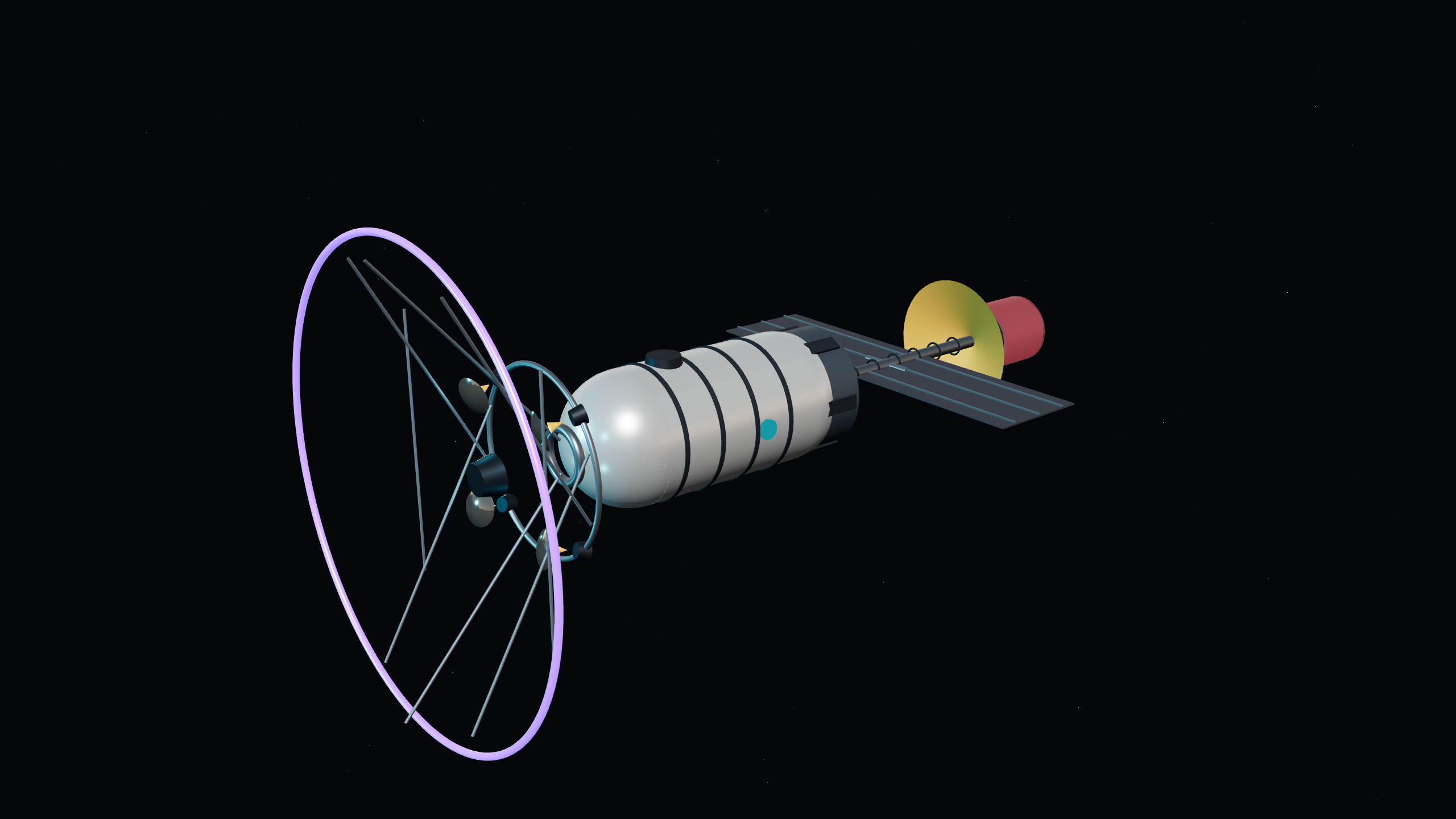
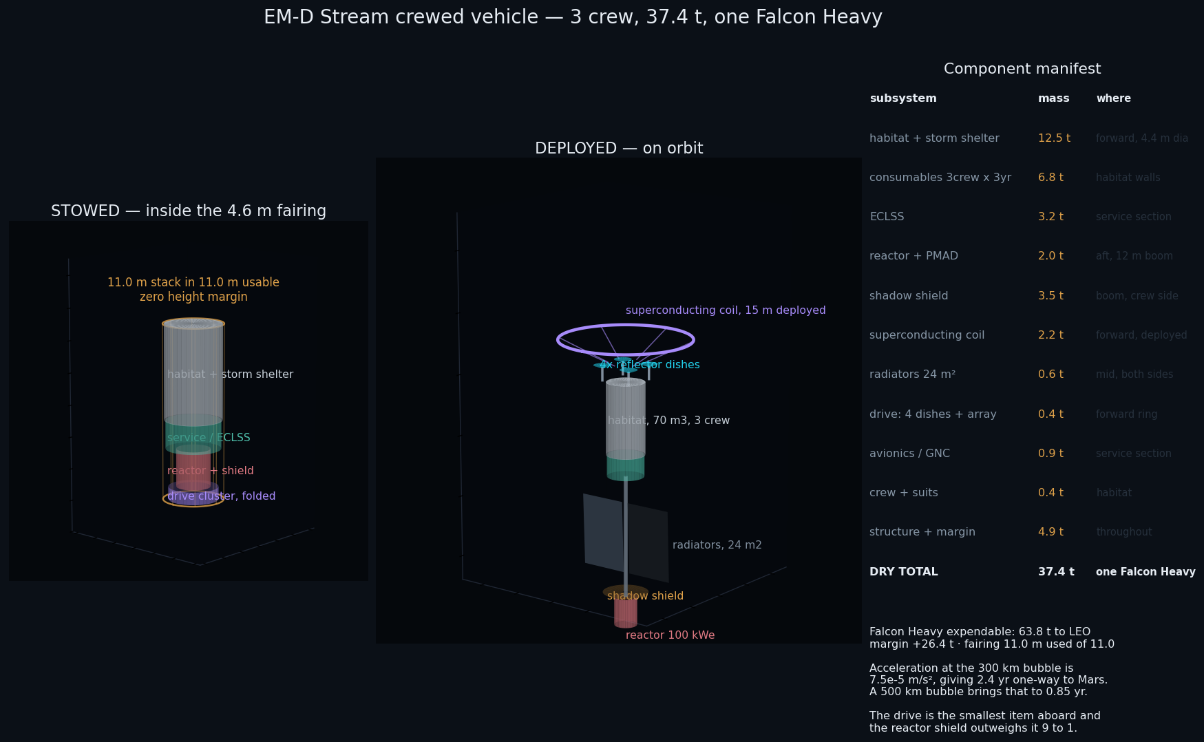
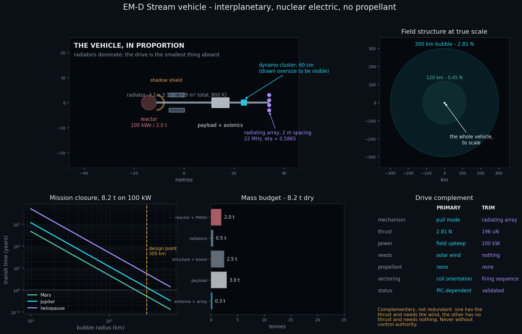
Rev C sized a 2.2 t superconducting coil to generate the magnetic moment directly, supported by a 100 kWe reactor, a shadow shield and radiators. That is not how the device works. The antenna does not generate the moment; it drives current in ambient plasma, and the plasma carries the moment. Rev D replaces the coil, reactor, shield and radiators with a 20 kg antenna, 120 kg of RMF power electronics, a 1 kW solar array and 40 kg of radiators. Power and drive fall from 8 700 kg to 240 kg, 36 times lighter. The crewed vehicle goes from 37.4 to 28.9 t, and the robotic probe from 8.2 to 0.9 t, its floor now set by structure and payload rather than by the drive.
| Subsystem | Mass | Where |
|---|---|---|
| Pressurised habitat structure | 8.5 t | forward, 4.4 m dia × 6.0 m |
| Storm shelter, water-walled | 4.0 t | inside the habitat |
| Consumables, 3 crew × 3 yr | 6.8 t | habitat walls |
| ECLSS, closed-loop | 3.2 t | service section |
| Avionics, comms, GNC | 900 kg | service section |
| Structure, docking, 15% margin | 4.9 t | throughout |
| Crew, suits, personal | 400 kg | habitat |
| RMF power electronics (drive) | 120 kg | service section |
| Solar array, 1 kW | 60 kg | service section, two wings |
| Radiators | 40 kg | service section, two panels |
| RMF antenna, 100 m radius | 20 kg | deployed loop, 100 W |
| Dry total | 28.9 t | one Falcon Heavy, expendable |
| Subsystem | Rev C | Rev D |
|---|---|---|
| Reactor + PMAD | 2 000 kg | removed |
| Shadow shield | 3 500 kg | removed |
| Radiators | 600 kg | 40 kg |
| Superconducting coil + cryo | 2 200 kg | removed |
| RMF antenna, 100 m | none | 20 kg |
| RMF power electronics | 400 kg | 120 kg |
| Solar array, 1 kW | none | 60 kg |
| Power + drive subtotal | 8 700 kg | 240 kg |
| Parameter | Value |
|---|---|
| Crew | 3 |
| Dry mass | 28.9 t (was 37.4 t in Rev C) |
| Launcher | Falcon Heavy, expendable (63.8 t to LEO) |
| Launch margin | +26.4 t |
| Stowed envelope | 11.0 m × 4.4 m diameter |
| Fairing usable | 11.0 m × 4.6 m, zero height margin |
| Habitable volume | 91.2 m³ gross, about 55 m³ net, 18.2 m³ per crew |
| Electrical power | 1 kW solar array, no reactor, no shield |
| RMF antenna | 100 m radius, 20 kg, 100 W (Slough point design) |
Mission performance
| Bubble | Thrust | Jet power | Probe 0.9 t, Mars | Crewed 28.9 t, Mars |
|---|---|---|---|---|
| 30 km (measured) | 3.78 N | 1.5 MW | 15 d | 495 d |
| 55 km (paper's 5 MW point) | 12.72 N | 5.1 MW | 5 d | 147 d |
| 100 km | 42.04 N | 16.8 MW | 1 d | 45 d |
| Leg | Duration |
|---|---|
| LEO escape | 22.9 d |
| Earth to Mars | 40.0 d |
| Mars capture | 15.0 d |
| Round trip with 30-day stay | 140 d |
Previous configuration and layout figures
Structural limit and component constraints
The hull is a pressure vessel loaded by its own field. Stress scales as m², which sets a ceiling on dynamo strength for a 2.2 m hull. The practical limit is about 3×10⁷ A·m² per dynamo for a 2.2 m aluminium hull.
| Moment per dynamo | Hoop stress | vs Al yield (270 MPa) | Verdict |
|---|---|---|---|
| 1×10⁶ A·m² | 0.04 MPa | 0.01% | acceptable |
| 1×10⁷ A·m² | 3.69 MPa | 1.4% | acceptable |
| 1×10⁸ A·m² | 369 MPa | 137% | hull fails |
| 3×10⁸ A·m² | 3317 MPa | 1229% | hull fails |
| Device | η_conv | N per kW electrical | Life (h) |
|---|---|---|---|
| Industrial CW magnetron | 0.85 | 2.764×10⁻⁶ | 5 000 |
| Klystron | 0.65 | 2.114×10⁻⁶ | about 20 000 |
| GaN solid-state amplifier | 0.60 | 1.951×10⁻⁶ | 100 000 |
Test article
| Item | Value |
|---|---|
| Dynamo separation | 15 cm, 4 units |
| Core volume | 5.0 litres; nulls at ±10.6 cm |
| Core field | 93 mT |
| Drive | pulsed 1 to 10 kHz, sub-μs sequenced delay |
| Plasma source | 10¹⁸ to 10¹⁹ m⁻³ |
| Instrument | torsion thrust balance |
| Predicted signal | 108 μN at 10¹⁸ / 1 kHz; 10.8 mN at 10¹⁹ / 10 kHz |
The sequential-firing result is testable on a bench without resolving any open item. The measurement is forward-minus-reverse: run the sequence in one order, then the other, and difference. Thrust must reverse; no other effect in the apparatus does. Thermal drift, outgassing, EMI and magnetic tare are all common-mode to sequence direction and cancel. The predicted signal sits two to four orders above a torsion balance's noise floor, which is what renders a null result meaningful.
Withdrawn claim: attitude authority
Rev C stated that the four-dynamo array supplies attitude authority the magnetic sail lacks. Quantitative check refutes this and the claim is withdrawn. The magsail attitude problem is real and acknowledged in the literature: the moment vector is stable perpendicular to the wind and a countervailing torque resists any other orientation. The alignment torque is \boldsymbol\tau = \mathbf m\times\mathbf B, and m is enormous by design.
| Bubble | τ required at 30° AoA | τ from array, 1 MW | Ratio |
|---|---|---|---|
| 10 km | 1.45×10³ N·m | 0.28 N·m | 1.9×10⁻⁴ |
| 55 km | 2.41×10⁵ N·m | 0.28 N·m | 1.2×10⁻⁶ |
| 120 km | 2.51×10⁶ N·m | 0.28 N·m | 1.1×10⁻⁷ |
Open problems
- 1 ScalingThe experiment used a 50 km/s laboratory wind source at high density. Flight is 400 km/s at about 10⁶ lower density. This is now the principal technical risk and replaces inflation as the headline unknown.
- 2 Constant-force claimSlough states the bubble expands as the wind thins, giving constant force with distance rather than the r^(−4/3) used throughout. At 30 AU that is a 96× difference. Unverified here.
- 3 Magsail steeringAcknowledged open in the literature. The withdrawn claim below establishes that the radiating array is not the answer.
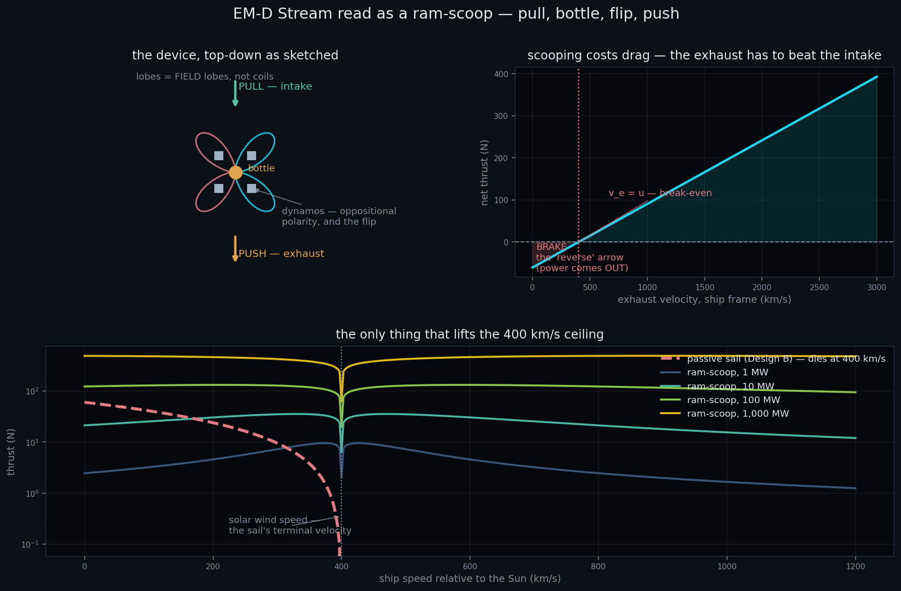
- 4 Exhaust velocity, drive C12.97 km/s against a 400 km/s wind, 31× short for ram-scoop operation.
- 5 Beam interception, charging, structural modesConventional spacecraft engineering, not computed.
| Item | Resolution |
|---|---|
| Plasma-magnet bubble inflation | > 10 kA driven, expansion demonstrated (Slough) |
| Plasmoid detachment | no detachment; force reacted onto the antennas |
Corrections register
| # | Previously | Corrected to | Cause |
|---|---|---|---|
| 1 | Alternating ring polarity | Aligned | alternating yields zero-measure null planes |
| 2 | Tension release as ejection | Sequential firing | breathing drives azimuthal E only |
| 3 | Counter-rotation cancels | η = 0.381 | earlier test sub-wavelength; artefact of scale |
| 4 | Scan covered handedness | It did not | rot_z never conjugates |
| 5 | 1 MW reactor | 100 kWe | sail is area-limited; 1 MW cost 18 t for nothing |
| 6 | Mission at 10 t, budget 29.8 t | Both 8.2 t | inconsistent mass |
| 7 | Thrust per kW radiated | Per kW electrical | 15 to 30% optimistic |
| 8 | Radiator for reactor only | Reactor + drive | magnetron loss uncounted |
| 9 | QUAD acceptance 3.17 m² | 0.000 m² | 3.75° grid counted a cell open from its edge |
| 10 | Sail thrust 0.45 N at 120 km | 60.5 N | used IMF magnetic pressure, not wind ram pressure; 134× |
| 11 | Habitat 70 m³, 14 m³ per crew | 91.2 m³, 18.2 m³ per crew | document figure contradicted its own source; found by audit |
| 12 | Crew and ship sizing used IMF pressure | ram pressure | 134× fix applied in one file but not propagated |
| 13 | Array gives magsail attitude authority | withdrawn | short by 10⁴ to 10⁷; τ = mB dwarfs photon torque |
| 14 | 2.2 t superconducting coil generates the moment | 20 kg RMF antenna drives plasma current | antenna is a transmitter, not a magnet; 36× lighter |
Downloads
Verification, the GPU integrator, the production run, the dimensional scan, reversibility, the asymptotic check, and the geodesic module. Appendices carry the full transcripts.
The document of record for the vehicle. Provenance, validated and negative results, physics, mechanism figures, the crewed configuration, structural limit, test article, withdrawn claim, open problems and the corrections register.
Complete derivations for the field topology, momentum transfer, the radiation bound, the circuit condition and hull loading. Written as a companion to Rev C (18 August 2026); where a number differs from Rev D, Rev D governs.
Bench article definition, measurement methodology, error budget, acceptance criteria, and the complete simulation record including every negative result. Pre-build: no hardware exists. Companion to Rev C.
Rev D is the document of record for the vehicle. The mathematical supplement and the test plan were written as companions to Rev C; where a number in them differs from Rev D, Rev D governs. The plasma-magnet measurements cited throughout are Slough (IEPC-2007-015, 2007).